Generalized linear models
Generalized Linear Models module of the GAMLj suite for jamovi
GAMLj version ≥ 1.6.0
The module estimates generalized linear models with categorial and/or continuous dependent and independent variables, with options to facilitate estimation ofinteractions, simple slopes, simple effects, etc.
Module
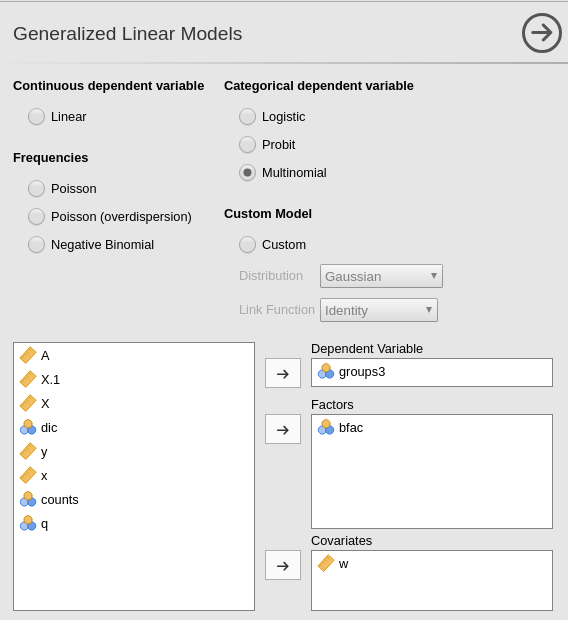
The module can estimate several linear models:
- Linear model
- Poisson model
- Poisson overdispersed
- Negative binomial model
- Logistic model
- Probit model
- Multinomial model
- Custom model with combinations of distribution and link function
For each model, any combination of categorical and continuous variables can be set as independent variables, thus providing an easy way for multiple regression, ANOVA-like, ANCOVA-like and moderation analysis for categorical and count dependent variables.
Models are defined by a link function (LF) and the dependent variable distribution, thus allowing to model different types of dependent variables:
Linear model: identity LF, gaussian distribution, yielding a general linear model for continuous dependent variables.
Poisson model: logarithm LF, Poisson distribution, modelling count dependent variables. This model is often called log-linear model when the independent variables are all categorical.
Poisson (overdispersion) model: Overdispersed Poisson model: logarithm LF, Poisson distribution, quasi-maximum likelihood estimation, with overdispersion, modelling count dependent variables. This model is often used for overdispersed data.
Negative binomial model: logarithm LF, negative binomial distribution, maximum likelihood estimation, with overdispersion, modelling count dependent variables. This model is often used for overdispersed data.
Logistic model: logit LF, binomial distribution, modelling dichotomous dependent variables.
Probit model: inverse of the cumulative normal distribution link function, binomial distribution, modelling dichotomous dependent variables.
Multinomial model: logit LF, multinomial distribution, modelling categorical dependent variables.
Custom model: combination of distribution family and link function.
The available distributions are:
- Gaussian
- Binomial
- Gamma
- Inverse Gaussian
The available link functions are:
- Identity
- Log
- Inverse
- Inverse squared
The plausibility of the distribution/link function combination is no checked, but errors are issued if the data do not conform to the chosen custom model.
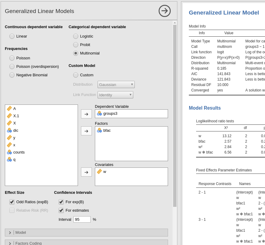
Estimates
The module provides Analysis of Deviance tables and parameter estimates for any estimated model. Variables definition follows jamovi standards, with categorical independent variables defined in “factors” and continuous independent variables in “covariates”.
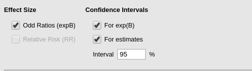
Effect size indexes are optionally computed by selecting
Odd rations (expB). Odd ratios apply the exponential
function to the parameter estimates, thus they make sense in all models
where the link function is based on the
logarithm.Relative risk (RR) indexes can be obtained for
logistic models.
Model
By default, the model terms are filled in automatically for main effects and for interactions with categorical variables.
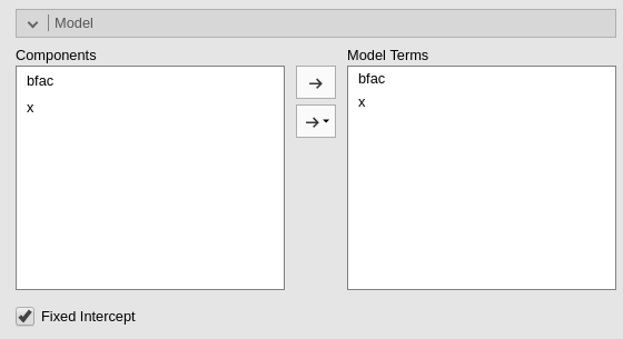
Interactions between continuous variables or categorical and continuous ones can be set by selecting one or more variables and clicking the second arrow icon.
Polinomial effects for continuous variables can be added to the model. When a variable is selected in the Components field, a little number appears on the right side of the selection. The number indicates the order of the effect.
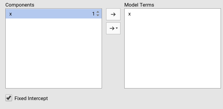
By increasing that number before dragging the term into the Model Terms field, one can include any high order effect.
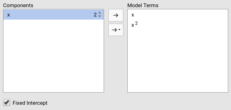
Increasing the order number and combining the selection with other variables allows including interactions involving higher order effects of a variable.
The option Fixed Intercept includes an intercept in the model. Unflag it to estimate zero-intercept models (Regression through the origin, but see here before you do it ).
Factors coding
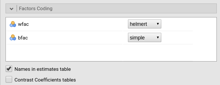
It allows to code the categorical variables according to different coding schemas. The coding schema applies to all parameters estimates. The default coding schema is simple, which is centered to zero and compares each means with the reference category mean. The reference category is the first appearing in the variable levels.
Note that all contrasts but dummy guarantee to be centered to zero (intercept being the grand mean), so when involved in interactions the other variables coefficients can be interpret as (main) average effects. If contrast dummy is set, the intercept and the effects of other variables in interactions are estimated for the first group of the categorical IV.
Contrasts definitions are provided in the estimates table. More detailed definitions of the comparisons operated by the contrasts can be obtained by selecting Show contrast definition table.
Differently to standard R naming system, contrasts variables are always named with the name of the factor and progressive numbers from 1 to K-1, where K is the number of levels of the factor.
In reading the contrast labels, one should interpret the
(1,2,3) code as meaning “the mean of the levels 1,2, and 3
pooled toghether”. If factor levels 1,2 and 3 are all levels of the
factor in the samples, (1,2,3) is equivalent to “the mean
of the sample”. For example, for a three levels factor, a contrast
labeled 1-(1,2,3) means that the contrast is comparing the
mean of level 1 against the mean of the sample. For the same factor, a
contrast labeled 1-(2,3) indicates a comparison between
level 1 mean and the subsequent levels means pooled together.
Covariates Scaling
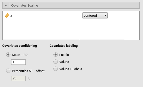
Continuous variables can be centered, standardized (z-scores), log-transformed (Log) or used as they are (none). The default is centered because it makes our lives much easier when there are interactions in the model, and do not affect the B coefficients when there are none. Thus, if one is comparing results with other software that does not center the continuous variables, without interactions in the model one would find only a discrepancy in the intercept, because in GAMLj the intercept represents the expected value of the dependent variable for the average value of the independent variable. If one needs to unscale the variable, simply select none.
Covariates conditioning rules how the model is conditioned to different values of the continuous independent variables in the simple effects estimation and in the plots when there is an interaction in the model.
Mean+SD: means that the IV is conditioned to the \(mean\), to \(mean+k \cdot sd\), and to \(mean-k\cdot sd\), where \(k\) is ruled by the white field below the option. Default is 1 SD.
Percentile 50 +offset: means that the IV is conditioned to the \(median\), the \(median+k P\), and the \(median-k\cdot P\), where \(P\) is the offset of percentile one needs. Again, the \(P\) is ruled by the white field below the option. Default is 25%. The default conditions the model to:
\(50^{th}-25^{th}=25^{th}\) percentile
\(50^{th}\) percentile
\(50^{th}+25^{th}=75^{th}\) percentile
The offset should be within 5 and 50.
Note that with either of these two options, one can estimate simple effects and plots for any value of the continuous IV.
Covariates labeling decides which label should be associated with the estimates and plots of simple effects as follows:
Labels produces strings of the form \(Mean \pm SD\)
Values uses the actual values of the variables
Labels+Values produces labels of the form \(Mean \pm SD=XXXX\), where
XXXXis the actual value.
Post-hocs
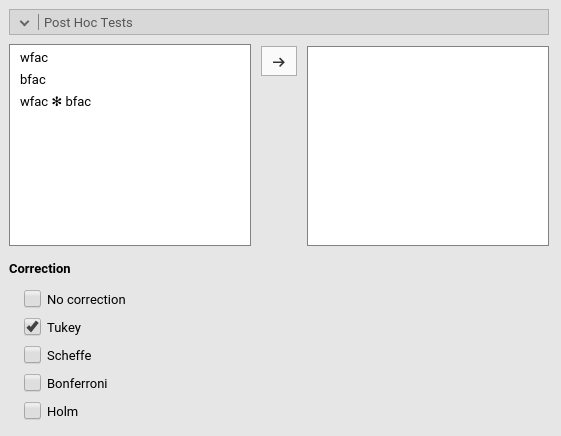
Post-hoc tests can be accomplished for the categorical variables groups by selecting the appropriated factor and flag the required tests
Post-hoc tests are implemented based on R package emmeans. All tecnical info can be found here
Plots
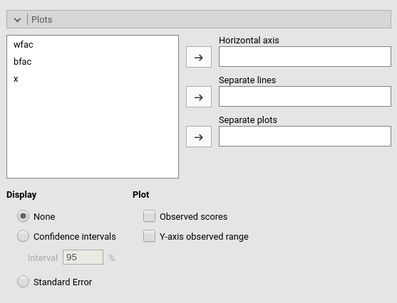
The “plots” menu allows for plotting main effects and interactions for any combination of types of variables, making it easy to plot interaction means plots, simple slopes, and combinations of them. The best plot is chosen automatically.
By filling in Horizontal axis one obtains the group means of the selected factor or the regression line for the selected covariate
By filling in Horizontal axis and Separated lines one obtains a different plot depending on the type of variables selected:
- Horizontal axis and Separated lines are both factors, one obtains the interaction plot of group means.
- Horizontal axis is a factor and Separated lines is a covariate. One obtains the plot of group means of the factor estimated at three different levels of the covariate. The levels are decided by the Covariates conditioning options above.
- Horizontal axis and Separated lines are covariates. One obtains the simple slopes graph of the simple slopes of the variable in horizontal axis estimated at three different levels of the covariate.
By filling in Separate plots one can
probe three-way interactions. If the selected variable is a factor, one
obtains a two-way graph (as previously defined) for each level of the
“Separate plots” variable. If the selected variable is a covariate, one
obtains a two-way graph (as previously defined) for the
Separate plots variable centered to conditioning values
selected in the Covariates conditioning
options.
Flagging the Display options add Confidence intervals (or confidence bands) or Standard errors to the plots.
Plot options allows to add observed data
to the plot (Observed scores) or to fix the
range of the plot to the actual range of the dependent variable (Y-axis observed range), without the need to plot
the actual predicted values. When Separate plots are
required, in each plot are showed only the observed scores of the
moderator level for which the plot is done when the moderator is a
categorical one, otherwise all data are plot in each plot.
Plots interpretation varies depending on the model being estimated. All plots are, however, depicting predicted values in the response original scale (usually probabilities). See details and interpretation discussion.
Estimated marginal means
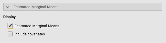
Print the estimate expected means, SE, df and confidence intervals of the precicted dependent variable by factors in the model. When `Include covariates is selected, factors levels are crossed also with the conditiong levels of the continuous variables (if any). The conditioning values are selected in Covariates Scaling panel.
Examples
Some worked out examples of the analyses carried out with jamovi GAMLj GZLM are posted here (more to come)
Details
Some more information about the module specs can be found here
Comments?
Got comments, issues or spotted a bug? Please open an issue on GAMLj at github or send me an email